Build Deep Learning Algorithms with TensorFlow 2.0, Dive into Neural Networks and Apply Your Skills in a Business Case.What you’ll learn
Requirements
Description Data scientists, machine learning engineers, and AI researchers all have their own skillsets. But what is that one special thing they have in common? They are all masters of deep learning. We often hear about AI, or self-driving cars, or the ‘algorithmic magic’ at Google, Facebook, and Amazon. But it is not magic – it is deep learning. And more specifically, it is usually deep neural networks – the one algorithm to rule them all. Cool, that sounds like a really important skill; how do I become a Master of Deep Learning? There are two routes you can take: The unguided route – This route will get you where you want to go, eventually, but expect to get lost a few times. If you are looking at this course you’ve maybe been there. The 365 route – Consider our route as the guided tour. We will take you to all the places you need, using the paths only the most experienced tour guides know about. We have extra knowledge you won’t get from reading those information boards and we give you this knowledge in fun and easy-to-digest methods to make sure it really sticks. Clearly, you can talk the talk, but can you walk the walk? – What exactly will I get out of this course that I can’t get anywhere else? Good question! We know how interesting Deep Learning is and we love it! However, we know that the goal here is career progression, that’s why our course is business focused and gives you real world practice on how to use Deep Learning to optimize business performance. We don’t just scratch the surface either – It’s not called ‘Skin-Deep’ Learning after all. We fully explain the theory from the mathematics behind the algorithms to the state-of-the-art initialization methods, plus so much more. Theory is no good without putting it into practice, is it? That’s why we give you plenty of opportunities to put this theory to use. Implement cutting edge optimizations, get hands on with TensorFlow and even build your very own algorithm and put it through training! Wow, that’s going to look great on your resume! Speaking of resumes, you also get a certificate upon completion which employers can verify that you have successfully finished a prestigious 365 Careers course – and one of our best at that! Now, I can see you’re bragging a little, but I admit you have peaked my interest. What else does your course offer that will make my resume shine? Trust us, after this course you’ll be able to fill your resume with skills and have plenty left over to show off at the interview.
This all sounds great, but I am a little overwhelmed, I’m afraid I may not have enough experience. We admit, you will need at least a little understanding of Python programming but nothing to worry about. We start with the basics and take you step by step toward building your very first (or second, or third etc.) Deep Learning algorithm – we program everything in Python and explain each line of code. We do this early on and it will give you the confidence to carry on to the more complex topics we cover. All the sophisticated concepts we teach are explained intuitively. Our beautifully animated videos and step by step approach ensures the course is a fun and engaging experience for all levels. We want everyone to get the most out of our course, and the best way to do that is to keep our students motivated. So, we worked hard to ensure that students with varying skills are challenged without being overwhelmed. Each lecture builds upon the last and practical exercises mean that you can practice what you’ve learned before moving on to the next step. And of course, we are available to answer any queries you have. In fact, we aim to answer any and all question within 1 business day. We don’t just chuck you in the pool then head to the bar and let you fend for yourself. Remember, we don’t just want you to enrol – we want you to complete the course and become a Master of Deep Learning. OK, awesome! I feel much better about my level of experience now, but we haven’t discussed yours! How do I know you can teach me to become a Master of Deep Learning? That’s an understandable worry, but it’s one we have no problem removing. We are 365 Careers and we’ve been creating online courses for ages. We have over 220,000 students and enjoy high ratings for all our Udemy courses. We are a team of experts who are all, at heart, teachers. We believe knowledge should be shared and not just through boring text books but in engaging and fun ways. We are well aware how difficult it is to build your knowledge and skills in the data science field, it’s so new and has grown so fast that the education sector has struggled to keep up and offer any substantial methods of teaching these topic areas. We wanted to change things – to rock the boat – so we developed our unique teaching style, one that countless students have enjoyed and thrived with. And between us, we think this course is one of our favourites, so if this is your first time with us, you’re in for a treat. If it’s not and you’ve taken one of our courses before, then, you’re still in for a treat! I’ve been hurt before though, how can I be sure you won’t let me down? Easy, with Udemy’s 30-day money back guarantee. We strive for the best and believe that our courses are the best out there. But you know what, everyone is different, and we understand that. So, we have no problem offering this guarantee, we want students who will complete and get the most out of this course. If you are one of the few who finds this course not what you wanted or expected then, get your money back. No questions, no risk, no problem. Great, that takes a load of my shoulders. What next? Click on the ‘Buy now’ button and take that first step toward a satisfying data science career and becoming a Master of Deep Learning. Who this course is for:
The post Deep Learning with TensorFlow 2.0 [2020] appeared first on Data Science PR. Originally from Machine Learning & AI – Data Science PR https://ift.tt/35rkJWV
0 Comments
New to machine learning? This is the place to start: Linear regression, Logistic regression & Cluster Analysis.What you’ll learn
Requirements
Description Are you an aspiring data scientist determined to achieve professional success? Are you ready and willing to master the most valuable skills that will skyrocket your data science career? Great! You’ve come to the right place. This course will provide you with the solid Machine Learning knowledge that will help you reach your dream job destination. That’s right. Machine Learning is one of the fundamental skills you need to become a data scientist. It is the stepping stone that will help you understand deep learning and modern data analysis techniques. In this course, we will explore the three most fundamental machine learning topics:
Surprised? Even neural networks geeks (like us) can’t help, but admit that it’s these 3 simple methods – linear regression, logistic regression and clustering that data science actually revolves around. So, in this course, we will make an otherwise complex subject matter easy to understand and apply in practice. Of course, there is only one way to teach these skills in the context of data science – to accompany statistics theory with practical application of these quantitative methods in Python. And that’s precisely what we are after. Theory and practice go hand in hand here. We have developed this course with not one but two machine learning libraries – StatsModels and sklearn. As our practical experience showed us, they have different use cases and should be used together rather than independently. Yet another advantage of taking this course? We are very conscious that data science theory is often overlooked.You can’t teach someone to run before they know how to walk. That’s why we will start slowly and continue by building complex ML models. But don’t assume you’ll be bored by theory. On the contrary! We have prepared a course that will get you results and will foster your interest in the subject matter, as it will show you that machine learning is something you can do, too (with the right teacher by your side). Well, we hope you are as excited as we are, as this course is the door that can open countless opportunities in the data science world for you. This is a course you’ll be actually eager to complete. On top of that we are happy to offer a 30-day money back guarantee. No risk for you. The content of the course is so outstanding , that this is a no-brainer for us We are 100% certain you will love it. Why wait any longer? Every day is a missed opportunity. Click the “Buy Now” button and let’s start (machine) learning together! Who this course is for:
Join now!The post Machine Learning 101 with Scikit-learn and StatsModels appeared first on Data Science PR. Originally from Machine Learning & AI – Data Science PR https://ift.tt/35aCkSX Acquire the #1 Skill Needed For Investment banking, Private equity, and Consulting – Company analysis.What you’ll learn
Requirements
Description ** Please be aware that this course is not an investment recommendation of any sort** What is the best way to learn financial modelling, valuation, corporate strategy, marketing fundamentals, and financial statement analysis? Go through a complete, real life case study. And which is arguably the hottest company in the business world today? Tesla Inc. This is the first online course attempting to teach several disciplines by combining them in a coherent and holistic case study of a company. In this course, we will touch on several important topics about Tesla:
Each topic we discuss is a natural continuation of what you have learned from the previous one. This will allow you to understand Tesla’s business very well. It is a fascinating firm that has already made huge steps towards achieving its mission: accelerate the world’s transition to sustainable energy. The entire auto industry is focused on electric vehicles, in large part because of how successful Tesla has been in the last few years. Tesla is a more expensive company than well-established traditional auto industry players like BMW and Daimler. And yet it sells 20x-30x fewer cars compared to these companies. According to investment banking analysts “Tesla has a brand following that is second only to Apple’s” However, many analysts are uncertain whether the company has sufficient cash to sustain its growth and win a bigger portion of the market? Tesla has established itself as the main innovator in the EV field. But its CEO, Elon Musk, decided to open-source all of the company’s patents. This is but one reason why Mr Musk is seen as the most exciting entrepreneur of this generation. While many feel he can do no wrong, he also runs multiple multibillion-dollar businesses and it is unclear how much time he is able to spend on Tesla. On our journey, we will encounter and analyse many contradictions surrounding Musk and Tesla. This is precisely what makes Tesla a perfect case study. Our goal with this course was to create a holistic, 360 degrees experience, that studies multiple facets of the company. We are not simply going to study financial statements. We will do that, but we will explore the company from multiple perspectives. Strategy:
Marketing:
Financial Statement Analysis:
Financial Modeling and Valuation:
This course is perfect for aspiring financial analysts, investment bankers, business analysts, consultants, or corporate executives. The skills you will acquire are the perfect blend of soft and technical skills that will give you an edge in interviews. This course comes with Udemy’s 30-day no questions asked money back guarantee. So, you have nothing to lose! Subscribe to the course and give it a try! Who this course is for:
Join now!The post Tesla Company Analysis: Strategy, Marketing, Financials appeared first on Data Science PR. Originally from Machine Learning & AI – Data Science PR https://ift.tt/2R77uCx When you first hear about regressions, you may think that correlation and regression are synonyms or at least they related to the same concept. This statement is somewhat supported by the fact that many academic papers in the past were based solely on correlations. However, correlation and regression are far from the same concept. So, let’s see what the relationship is between correlation analysis and regression analysis. There is a single expression that sums it up nicely: correlation does not imply causation! With that in mind, it’s time to start exploring the various differences between correlation and regression. 1. The Relationship between VariablesFirst, correlation measures the degree of relationship between two variables. Regression analysis is about how one variable affects another or what changes it triggers in the other. 
For more on variables and regression, check out our tutorial How to Include Dummy Variables into a Regression. 2. CausalitySecond, correlation doesn’t capture causality but the degree of interrelation between the two variables. Regression is based on causality. It shows no degree of connection, but cause and effect. 
3. Are X and Y Interchangeable?Third, a property of correlation is that the correlation between x and y is the same as between y and x. You can easily spot that from the formula, which is symmetrical. Regressions of y on x and x on y yield different results. Think about income and education. Predicting income, based on education makes sense, but the opposite does not. 
4. Graphical Representation of Correlation and Regression AnalysisFinally, the two methods have a very different graphical representation. Linear regression analysis is known for the best fitting line that goes through the data points and minimizes the distance between them. Whereas, correlation is a single point. 
Want to learn how to visualize statistical data? Check out our tutorials How to Visualize Numerical Data with Histograms and Visualizing Data with Bar, Pie and Pareto Charts. Key Differences Between Correlation and RegressionTo sum up, there are four key aspects in which these terms differ.
So, now that you have proof that correlation and regression are different, it is time for a new challenge. Find out how to decompose variability by diving into the linked tutorial. The article first appeared on: https://365datascience.com/correlation-regression/ The post The Difference between Correlation and Regression Explained in 2020 appeared first on Data Science PR. Originally from Machine Learning & AI – Data Science PR https://ift.tt/2EI2ykZ The word standardization may sound a little weird at first but understanding it in the context of statistics is not brain surgery. It is something that has to do with distributions. In fact, every distribution can be standardized. Say the mean and the variance of a variable are mu and sigma squared respectively. Standardization is the process of transforming a variable to one with a mean of 0 and a standard deviation of 1. You can see how everything is denoted below along with the formula that allows us to standardize a distribution. 
Standard Normal Distribution in Statistics: Definition and FormulasLogically, a normal distribution can also be standardized. The result is called a standard normal distribution. 
You may be wondering how the standardization goes down here. Well, all we need to do is simply shift the mean by mu, and the standard deviation by sigma. 
We use the letter Z to denote it. As we already mentioned, its mean is 0 and its standard deviation: 1. 
The standardized variable is called a z-score. It is equal to the original variable, minus its mean, divided by its standard deviation. 
A Case in PointLet’s take an approximately normally distributed set of numbers: 1, 2, 2, 3, 3, 3, 4, 4, and 5. 
Its mean is 3 and its standard deviation: 1.22. Now, let’s subtract the mean from all data points. As shown below, we get a new data set of: -2, -1, -1, 0, 0, 0, 1, 1, and 2. 
The new mean is 0, exactly as we anticipated. 
Showing that on a graph, we have shifted the curve to the left, while preserving its shape. The Next Step of the StandardizationSo far, we have a new distribution. It is still normal, but with a mean of 0 and a standard deviation of 1.22. The next step of the standardization is to divide all data points by the standard deviation. This will drive the standard deviation of the new data set to 1. Let’s go back to our example. The original dataset has a standard deviation of 1.22. The same goes for the dataset which we obtained after subtracting the mean from each data point. 
Important: Adding and subtracting values to all data points does not change the standard deviation. Now, let’s divide each data point by 1.22. As you can see in the picture below, we get: -1.6, -0.82, -0.82, 0, 0, 0, 0.82, 0.82, and 1.63. 
If we calculate the standard deviation of this new data set, we will get 1. And the mean is still 0! 
In terms of the curve, we kept it at the same position, but reshaped it a bit, as shown below. 
Standardization of Normal Distribution: Next StepsThis is how we can obtain a standard normal distribution from any normally distributed data set. Using it makes predictions and inferences much easier. This is exactly what will help us a great deal in the next tutorials. So, if you want to use the knowledge you gained here, feel free to jump into the linked tutorial. The article first appeared on: https://365datascience.com/standardization/ The post Obtaining Standard Normal Distribution Step-By-Step Guide in 2020 appeared first on Data Science PR. Originally from Machine Learning & AI – Data Science PR https://ift.tt/32QcgK0 If you want to become a better statistician, a data scientist, or a machine learning engineer, going over several linear regression examples is inevitable. They will help you to wrap your head around the whole subject of regressions analysis. 
Regression analysis is one of the most widely used methods for prediction. It is applied whenever we have a causal relationship between variables. 
A large portion of the predictive modeling that occurs in practice is carried out through regression analysis. There are also many academic papers based on it. And it becomes extremely powerful when combined with techniques like factor analysis. Moreover, the fundamentals of regression analysis are used in machine learning. 
Therefore, it is easy to see why regressions are a must for data science. The general point is the following.

In the same way, the amount of time you spend reading our tutorials is affected by your motivation to learn additional statistical methods. 
You can quantify these relationships and many others using regression analysis. Regression AnalysisWe will use our typical step-by-step approach. We’ll start with the simple linear regression model, and not long after, we’ll be dealing with the multiple regression model. Along the way, we will learn how to build a regression, how to interpret it and how to compare different models. 
We will also develop a deep understanding of the fundamentals by going over some linear regression examples. A quick side note: You can learn more about the geometrical representation of the simple linear regression model in the linked tutorial. What is a Linear RegressionLet’s start with some dry theory. A linear regression is a linear approximation of a causal relationship between two or more variables. 
Regression models are highly valuable, as they are one of the most common ways to make inferences and predictions. The Process of Creating a Linear RegressionThe process goes like this.

There is a dependent variable, labeled Y, being predicted, and independent variables, labeled x1, x2, and so forth. These are the predictors. Y is a function of the X variables, and the regression model is a linear approximation of this function. 
The Simple Linear RegressionThe easiest regression model is the simple linear regression: Y = β0 + β1 * x1 + ε. Let’s see what these values mean. Y is the variable we are trying to predict and is called the dependent variable. X is an independent variable. 
When using regression analysis, we want to predict the value of Y, provided we have the value of X. But to have a regression, Y must depend on X in some way. Whenever there is a change in X, such change must translate to a change in Y. Providing a Linear Regression ExampleThink about the following equation: the income a person receives depends on the number of years of education that person has received. The dependent variable is income, while the independent variable is years of education. 
There is a causal relationship between the two. The more education you get, the higher the income you are likely to receive. This relationship is so trivial that it is probably the reason you are reading this tutorial, right now. You want to get a higher income, so you are increasing your education. 
Is the Reverse Relationship Possible?Now, let’s pause for a second and think about the reverse relationship. What if education depends on income. 
This would mean the higher your income, the more years you spend educating yourself. 
Putting high tuition fees aside, wealthier individuals don’t spend more years in school. Moreover, high school and college take the same number of years, no matter your tax bracket. Therefore, a causal relationship like this one is faulty, if not plain wrong. Hence, it is unfit for regression analysis. 
Let’s go back to the original linear regression example. Income is a function of education. The more years you study, the higher the income you will receive. This sounds about right. 
The CoefficientsWhat we haven’t mentioned, so far, is that, in our model, there are coefficients. β1is the coefficient that stands before the independent variable. It quantifies the effect of education on income. 
If β1 is 50, then for each additional year of education, your income would grow by $50. In the USA, the number is much bigger, somewhere around 3 to 5 thousand dollars. 
The ConstantThe other two components are the constant β0 and the error – epsilon(ε). In this linear regression example, you can think of the constant β0 as the minimum wage. No matter your education, if you have a job, you will get the minimum wage. This is a guaranteed amount. So, if you never went to school and plug an education value of 0 years in the formula, what could possibly happen? Logically, the regression will predict that your income will be the minimum wage. 
EpsilonThe last term is the epsilon(ε). This represents the error of estimation. The error is the actual difference between the observed income and the income the regression predicted. On average, across all observations, the error is 0. 
If you earn more than what the regression has predicted, then someone earns less than what the regression predicted. Everything evens out. The Linear Regression EquationThe original formula was written with Greek letters. This tells us that it was the population formula. But don’t forget that statistics (and data science) is all about sample data. In practice, we tend to use the linear regression equation. It is simply ŷ = β0+ β1* x. 
The ŷ here is referred to as y hat. Whenever we have a hat symbol, it is an estimated or predicted value. B0 is the estimate of the regression constant β0. Whereas, b1 is the estimate of β1, and x is the sample data for the independent variable. The Regression LineYou may have heard about the regression line, too. When we plot the data points on an x-y plane, the regression line is the best-fitting line through the data points. 
You can take a look at a plot with some data points in the picture above. We plot the line based on the regression equation. The grey points that are scattered are the observed values. B0, as we said earlier, is a constant and is the intercept of the regression line with the y-axis. 
B1 is the slope of the regression line. It shows how much y changes for each unit change of x. 
The Estimator of the ErrorThe distance between the observed values and the regression line is the estimator of the error term epsilon. Its point estimate is called residual. 
Now, suppose we draw a perpendicular from an observed point to the regression line. The intercept between that perpendicular and the regression line will be a point with a y value equal to ŷ. 
As we said earlier, given an x, ŷ is the value predicted by the regression line. 
Linear Regression in Python ExampleWe believe it is high time that we actually got down to it and wrote some code! So, let’s get our hands dirty with our first linear regression example in Python. If this is your first time hearing about Python, don’t worry. We have plenty of tutorials that will give you the base you need to use it for data science and machine learning. Now, how about we write some code? First off, we will need to use a few libraries. Importing the Relevant LibrariesLet’s import the following libraries: 
The first three are pretty conventional. We won’t even need numpy, but it’s always good to have it there – ready to lend a helping hand for some operations. In addition, the machine learning library we will employ for this linear regression example is: statsmodels. So, we can basically write the following code: import numpy as np
Loading the DataThe data which we will be using for our linear regression example is in a .csv file called: ‘1.01. Simple linear regression.csv’. You can download it from here. Make sure that you save it in the folder of the user. Now, let’s load it in a new variable called: data using the pandas method: ‘read_csv’. We can write the following code:
After running it, the data from the .csv file will be loaded in the data variable. As we are using pandas, the data variable will be automatically converted into a data frame. 
Visualizing the Data FrameLet’s see if that’s true. We can write data and run the line. As you can see below, we have indeed displayed the data frame. 
There are two columns – SAT and GPA. And that’s what our linear regression example will be all about. Let’s further check
This is a pandas method which will give us the most useful descriptive statistics for each column in the data frame – number of observations, mean, standard deviation, and so on. 
In this linear regression example we won’t put that to work just yet. However, it’s good practice to use it. The ProblemLet’s explore the problem with our linear regression example. So, we have a sample of 84 students, who have studied in college. 
Their total SAT scores include critical reading, mathematics, and writing. Whereas, the GPA is their Grade Point Average they had at graduation. 
That’s a very famous relationship. We will create a linear regression which predicts the GPA of a student based on their SAT score. When you think about it, it totally makes sense.
You can see the timeline below. 
Meaningful RegressionsBefore we finish this introduction, we want to get this out of the way. Each time we create a regression, it should be meaningful. Why would we predict GPA with SAT? Well, the SAT is considered one of the best estimators of intellectual capacity and capability. On average, if you did well on your SAT, you will do well in college and at the workplace. Furthermore, almost all colleges across the USA are using the SAT as a proxy for admission. And last but not least, the SAT stood the test of time and established itself as the leading exam for college admission. 
It is safe to say our regression makes sense. Creating our First Regression in PythonAfter we’ve cleared things up, we can start creating our first regression in Python. We will go through the code and in subsequent tutorials, we will clarify each point. Important: Remember, the equation is: Our dependent variable is GPA, so let’s create a variable called y which will contain GPA. Just a reminder – the pandas’ syntax is quite simple. This is all we need to code:
It goes like this:
Similarly, our independent variable is SAT, and we can load it in a variable x1. 
Exploring the DataIt’s always useful to plot our data in order to understand it better and see if there is a relationship to be found. We will use some conventional matplotlib code.
You can see the result we receive after running it, in the picture below. 
Each point on the graph represents a different student. For instance, the highlighted point below is a student who scored around 1900 on the SAT and graduated with a 3.4 GPA. 
Observing all data points, we can see that there is a strong relationship between SAT and GPA. In general, the higher the SAT of a student, the higher their GPA. 
Adding a ConstantNext, we need to create a new variable, which we’ll call x. We have our x1, but we don’t have an x0. In fact, in the regression equation there is no explicit x0. The coefficient b0 is alone. 
That can be represented as: b0 * 1. So, if there was an x0, it would always be 1. 
It is really practical for computational purposes to incorporate this notion into the equation. And that’s how we estimate the intercept b0. In terms of code, statsmodels uses the method: .add_constant(). So, let’s declare a new variable:
The Results VariableRight after we do that, we will create another variable named results. It will contain the output of the ordinary least squares regression, or OLS. As arguments, we must add the dependent variable y and the newly defined x. At the end, we will need the .fit() method. It is a method that applies a specific estimation technique to obtain the fit of the model. 
That itself is enough to perform the regression. Displaying the Regression ResultsIn any case, results.summary() will display the regression results and organize them into three tables. So, this is all the code we need to run:
And this is what we get after running it: 
As you can see, we have a lot of statistics in front of us! And we will examine it in more detail in subsequent tutorials. Plotting the Regression lineLet’s plot the regression line on the same scatter plot. We can achieve that by writing the following:
As you can see below, that is the best fitting line, or in other words – the line which is closest to all observations simultaneously. 
So that’s how you create a simple linear regression in Python! How to Interpret the Regression TableNow, let’s figure out how to interpret the regression table we saw earlier in our linear regression example. While the graphs we have seen so far are nice and easy to understand. When you perform regression analysis, you’ll find something different than a scatter plot with a regression line. The graph is a visual representation, and what we really want is the equation of the model, and a measure of its significance and explanatory power. This is why the regression summary consists of a few tables, instead of a graph. 
Let’s find out how to read and understand these tables. The 3 Main TablesTypically, when using statsmodels, we’ll have three main tables – a model summary 
a coefficients table 
and some additional tests. 
Certainly, these tables contain a lot of information, but we will focus on the most important parts. We will start with the coefficients table. The Coefficients TableWe can see the coefficient of the intercept, or the constant as they’ve named it in our case. 
Both terms are used interchangeably. In any case, it is 0.275, which means b0 is 0.275. 
Looking below it, we notice the other coefficient is 0.0017. This is our b1. These are the only two numbers we need to define the regression equation. 
Therefore, ŷ= 0.275 + 0.0017 * x1. Or GPA equals 0.275 plus 0.0017 times SAT score. 
So, this is how we obtain the regression equation. A Quick RecapLet’s take a step back and look at the code where we plotted the regression line. We have plotted the scatter plot of SAT and GPA. That’s clear. After that, we created a variable called: y hat(ŷ). Moreover, we imported the seaborn library as a ‘skin’ for matplotlib. We did that in order to display the regression in a prettier way. 
That’s the regression line – the predicted variables based on the data. 
Finally, we plot that line using the plot method. 
Naturally, we picked the coefficients from the coefficients table – we didn’t make them up. The Predictive Power of Linear RegressionsYou might be wondering if that prediction is useful. Well, knowing that a person has scored 1700 on the SAT, we can substitute in the equation and obtain the following: 0.275 + 0.0017 * 1700, which equals 3.165. So, the expected GPA for this student, according to our model is 3.165. 
And that’s the predictive power of linear regressions in a nutshell! The Standard ErrorsWhat about the other cells in the table? The standard errors show the accuracy of prediction for each variable. The lower the standard error, the better the estimate! 
The T-StatisticThe next two values are a T-statistic and its P-value. 
If you have gone over our other tutorials, you may know that there is a hypothesis involved here. The null hypothesis of this test is: β = 0. In other words, is the coefficient equal to zero? 
The Null HypothesisIf a coefficient is zero for the intercept(b0), then the line crosses the y-axis at the origin. You can get a better understanding of what we are talking about, from the picture below. 
If β1is zero, then 0 * x will always be 0 for any x, so this variable will not be considered for the model. Graphically, that would mean that the regression line is horizontal – always going through the intercept value. 
The P-ValueLet’s paraphrase this test. Essentially, it asks, is this a useful variable? Does it help us explain the variability we have in this case? The answer is contained in the P-value column. 
As you may know, a P-value below 0.05 means that the variable is significant. Therefore, the coefficient is most probably different from 0. Moreover, we are longing to see those three zeroes. 
What does this mean for our linear regression example? Well, it simply tells us that SAT score is a significant variable when predicting college GPA. What you may notice is that the intercept p-value is not zero. 
Let’s think about this. Does it matter that much? This test is asking the question: Graphically, that would mean that the regression line passes through the origin of the graph. 
Usually, this is not essential, as it is causal relationship of the Xs we are interested in. The F-statisticThe last measure we will discuss is the F-statistic. We will explain its essence and see how it can be useful to us. 
Much like the Z-statistic which follows a normal distribution and the T-statistic that follows a Student’s T distribution, the F-statistic follows an F distribution. 
We are calling it a statistic, which means that it is used for tests. The test is known as the test for overall significance of the model. The Null Hypothesis and the Alternative HypothesisThe null hypothesis is: all the βs are equal to zero simultaneously. The alternative hypothesis is: at least one β differs from zero. 
This is the interpretation: if all βs are zero, then none of the independent variables matter. Therefore, our model has no merit. In our case, the F-statistic is 56.05. 
The cell below is its P-value. 
As you can see, the number is really low – it is virtually 0.000. We say the overall model is significant. Important: Notice how the P-value is a universal measure for all tests. There is an F-table used for the F-statistic, but we don’t need it, because the P-value notion is so powerful. The F-test is important for regressions, as it gives us some important insights. Remember, the lower the F-statistic, the closer to a non-significant model. Moreover, don’t forget to look for the three zeroes after the dot! Create Your Own Linear RegressionsWell, that was a long journey, wasn’t it? We embarked on it by first learning about what a linear regression is. Then, we went over the process of creating one. We also went over a linear regression example. Afterwards, we talked about the simple linear regression where we introduced the linear regression equation. By then, we were done with the theory and got our hands on the keyboard and explored another linear regression example in Python! We imported the relevant libraries and loaded the data. We cleared up when exactly we need to create regressions and started creating our own. The process consisted of several steps which, now, you should be able to perform with ease. Afterwards, we began interpreting the regression table. We mainly discussed the coefficients table. Lastly, we explained why the F-statistic is so important for regressions. Next Step: CorrelationYou thought that was all you need to know about regressions? Well, seeing a few linear regression examples is not enough. There are many more skills you need to acquire in order to truly understand how to work with linear regressions. The first thing which you can clear up is the misconception that regression and correlation are referring to the same concept. Article first appeared on: https://365datascience.com/linear-regression/ The post How To Perform A Linear Regression In Python in 2020 appeared first on Data Science PR. Originally from Machine Learning & AI – Data Science PR https://ift.tt/3jErU1G In this post, we will focus on removing records from a database. This operation is carried out with the SQL DELETE statement. Before reading this tutorial be sure to check out our posts on SQL UPDATE Statement and SQL INSERT Statement. Executing an SQL DELETE statementFollowing what we said in the previous post regarding COMMIT and ROLLBACK, and knowing that in this post we are about to delete items, we will start by executing a COMMIT. Thus, we will store the current state of our database. If necessary, we will be able to revert to it later using ROLLBACK. 
In the post about INSERT, under employee number 9-9-9-9-0-3 we added some information about Jonathan Creek. Let’s select his record in the “Employees” table. 
Fine – we can see his ‘birthdate’, ‘gender’ and ‘hire date’. Now, let’s see what information is contained about the same employee in the “Titles” table. 
Excellent! His job position is ‘senior engineer’, and he started working on the 1st of October 1997. The lack of information in the “to_date” column suggests that he is still working at the company. Good! As we mentioned at the beginning of the tutorial, the syntax to abide by when deleting information is DELETE FROM, table name, and WHERE with a corresponding condition. 
In our case, the code would be DELETE FROM “Employees”, WHERE “Employee number” is 9-9-9-9-0-3. 
What should happen when we run this query is that only the row with employee number 9-9-9-9-0-3 will be removed. Let’s see if this is true after executing this DELETE statement, then selecting the record from the “Employees” table, providing the same condition in the WHERE clause. 
So … what output will show up? 
An empty record. This means we have properly deleted the information about Jonathan Creek. Awesome! What do you think … can we still see he was a senior engineer hired in October 1997? We’ll have to check what’s left in the “Titles” table. 
Hmm … empty as well. Why? Didn’t we order a DELETE command for only the “Employees” table? The answer lies in the connection between the two tables. 
Then we check the DDL information about the “Titles” table. 
We see in the foreign key constraint that we also have an ON DELETE CASCADE clause. 
Using this clause means all related records in the child table will be deleted as well. Fantastic! For the sake of exercise, assume we deleted Jonathan’s information by mistake. Is there a way we can go back? Considering that we applied a COMMIT statement at the beginning of the post, then, yes, there is. We should be able to run a ROLLBACK command. Let’s execute it … ok! 
And now let’s verify that the record has been put back in the table. It’s in the “Employees” table … ok… 
And … we have it in “Titles”, too. 
So, our last COMMIT did a good job preserving the full dataset – the initial large data set along with the three records we added in the INSERT section. Keep up the pace for the next section, in which we’ll show you something with which you must be very careful. Unsafe Delete OperationIf we do not set a condition in the WHERE clause of a DELETE statement, we are taking a big risk. This could potentially lead to the removal of all the table’s records. That’s why we must be very careful when using this statement. Always! 
Let’s recall what we have in the “Departments Duplicate” table. 
The numbers and names of nine departments in the company. Let’s execute a DELETE statement without a WHERE clause attached to it. 
You see? Nine rows were affected. 
Now we can check the table once more. 
It couldn’t be emptier than that! To undo the changes, we should be able to execute a ROLLBACK statement. Ok? 
And … did it work? We’ll have to select all the information from this tiny table to verify whether we have our data back. 
Here it is! Waiting to be retrieved! Therefore, in conclusion, we can say the following: Be careful with the DELETE statement. Don’t forget to attach a condition in the WHERE clause unless you want to lose all your information. In the next section, we will compare DROP, DELETE, and TRUNCATE. DROP vs TRUNCATE vs DELETEIn this section, we will briefly discuss the main difference between three reserved words: DROP, TRUNCATE, and DELETE. Their functionality is similar, and you might wonder why all of them – and not just one – exist. DROP
Look at this hypothetical table with 10 records. If you DROP it, you will lose the records, the table as a structure, and all related objects, like indexes and constraints. You will lose everything! Furthermore, you won’t be able to roll back to its initial state, or to the last COMMIT statement. Once you drop a table, it’s gone. Only additional data recovery software will help in such a situation, but it is not considered a standard SQL tool. Hence, use DROP TABLE only when you are sure you aren’t going to use the table in question anymore. TRUNCATE
TRUNCATE is a statement that will essentially remove all records from the table, just as if you had used DELETE without a WHERE clause. This means TRUNCATE will remove all records in your table, but its structure will remain intact. Please bear in mind that when truncating, auto-increment values will be reset. So, if your table has 10 records and then you truncate it, when you start re-filling this data object with information, the next records that will be inserted are not going to be 11 and 12. The first record will be number 1, the second record will be number 2, and so on. Nice! 
DELETEFinally, DELETE removes records row by row. Only the rows corresponding to a certain condition, or conditions, specified in the WHERE clause will be deleted. 
If the WHERE block is omitted, the output will resemble the one obtained with TRUNCATE. There will be a couple of significant distinctions, though. First, the SQL optimizer will implement different programmatic approaches when we are using TRUNCATE or DELETE. As a result, TRUNCATE delivers the output much quicker than DELETE because it does not need to remove information row by row. Second, auto-increment values are not reset with DELETE. So, if you DELETE all 10 records in this table and then start inserting new data, the first new record will be numbered 11, and not 1; the second will be 12, and not 2, and so on. 
There are many other technical peculiarities regarding these three options but their detailed explanation is beyond the scope of this post. Nevertheless, we hope this post will help you make a more educated choice among DROP, TRUNCATE, and DELETE. To learn more about SQL statements, check out our tutorials How to Use the Limit Statement in SQL and When to Use the SQL CASE Statement. You can also watch our explainer videos or simply continue to the next tutorial to understand how to manipulate data and use operators in SQL. The article first appeared on: https://365datascience.com/sql-delete-statement/ The post SQL DELETE Statement Explained appeared first on Data Science PR. Originally from Machine Learning & AI – Data Science PR https://ift.tt/32KijzE We’re now entering the concept of relationships between tables in SQL. You will feel more comfortable reading this tutorial if you are familiar with and the primary, foreign and unique keys. This is a tutorial in which we will illustrate that these relationships can be categorized. We will not explore all types in detail given that this topic is rather theoretical and time-consuming in its entirety. Instead, we will study the main types of relationships between the tables you will likely need in your workplace. 
Types of RelationshipsRelationships between tables tell you how much of the data from a foreign key field can be seen in the related primary key column and vice versa. 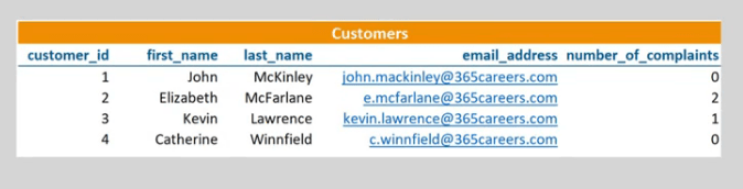
As you can see in the picture above, the “customer_id” column is a primary key of the “Customers” table. This means it contains only unique values – 1, 2, 3, and 4. The same information about “customer_id” can be found in a table called “Sales” as a foreign key, but you will likely have a lot more than 4 rows there. 
Hence, the values from 1 to 4 can be repeated many times because the same customer can execute more than one purchase. One-to-Many RelationshipThis is an example of a ‘one-to-many’ type of relationship: one value from the “customer_id” column in the “Customers” table can be found many times in the “customer_id” column in the “Sales” table. As a relational schema, this is shown by assigning the correct symbols at the end of the arrow. 
How to Display the RelationshipYou should always read the symbols according to the direction of the relationship you are exploring. The First DirectionFor instance, think of it this way: a single customer could have made one purchase, but he could have also made multiple! Therefore, the second symbol, which is next to the rectangle, shows the minimum number of instances of the “Customers” entity that can be associated with the “Sales” entity. 
When this symbol is a tiny line, it means “one”. The symbol located next to the rectangle indicates the maximum number of instances that can be associated with the “Sales” entity. The angle-like symbol stands for “many”. 
The Opposite DirectionLet’s check the relationship in the opposite direction. For a single purchase registered in the “Sales” table a single customer can be indicated as the buyer. So, we must have the name, email and number of complaints for at least one customer in the “Customers” table that corresponds to a single purchase in the “Sales” table. Therefore, the minimum number is 1. 
At the same time, we just mentioned that for a given purchase we cannot have more than one buyer, meaning that the maximum number of instances from “Sales” associated with “Customers” is also one. Hence, for every purchase, we can obtain the name, email, and number of complaints data for one customer, and we represent this logic by drawing а line for the minimum, and а line for the maximum. 
Cardinality ConstraintsThe two symbols in closer proximity to the rectangles form the relationship between the “Customers” and the “Sales” tables. In our case, it is correct to say that the “Customers” to “Sales” relationship is one-to-many, while “Sales” to “Customers” is many-to-one. The symbols showing us relationship limitations are called cardinality constraints. There are other symbols that can be used too. ‘M’ or ‘N’ for infinite associations, or a circle for optional instances. The latter would have been the case if it weren’t necessary for a registered person to have purchased an item. 
More Types of RelationshipsThere are some other types of relationships between tables as well – one-to-one, many-to-many, etc. This is information that we share with you as general knowledge. This is a specialized topic which is of interest mainly to advanced users. Why We Use Relational SchemasIn summary, relational (or database) schemas do not just represent the concept database administrators must implement. They depict how a database is organized. They can be thought of as blueprints, or a plan for a database, because they are usually prepared at the stage of a database’s design. 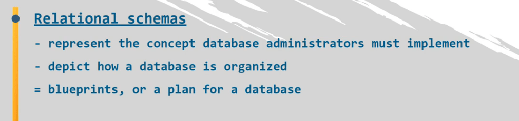
Drawing a relational schema isn’t an easy job, but relational schemas will help you immensely while writing your queries. A neat and complete visualization of the structure of the entire database will always be useful for retrieving information. Presenting Relationships between Tables in SQLTo conclude, we display relationships between tables in SQL with cardinality constraints because it makes it easier to understand. Now, that you know how they are used; you can figure out the category of a relationship by simply looking at the database schema. The next step will be to learn how to install and use the MySQL Workbench. Article first appeared on: https://365datascience.com/sql-relationships-between-tables/ The post Relationships between Tables in SQL in 2020 appeared first on Data Science PR. Originally from Machine Learning & AI – Data Science PR https://ift.tt/3513yev So, you want to learn how to code in Python? Well, you can’t do that without knowing how to work with Python functions. No worries though, in this tutorial we’ll teach you how to use Python functions and how these can help you when programming in Python. The best way of learning is by doing, so let’s create our first function and see how it can be applied. How to Define a Function in Python?

For instance, simple, as we will create a very simple function. Then we can add a pair of parentheses. Technically, within these parentheses, you could place the parameters of the function if it requires you to have any. It is no problem to have a function with zero parameters. This is the case with the function we are creating right now. To proceed, don’t forget to add a colon after the name of the function. Since it is inconvenient to continue on the same line when the function becomes longer, it is much better to build the habit of laying the instructions on a new line, with an indent again. Good legibility counts for а good style of coding! And fewer arguments with the people you are working with (those wise guys…) 
All right, let’s see what will happen when we ask the machine to print a sentence. 
Not much, at least for now. The computer created the function “simple” that can print out “My first function”, but that was all. To apply the function, we must call it. We must ask the function to do its job. So, we will obtain its result once we type its name, “simple”, and parentheses. See? 
Great! Let’s do something a bit more sophisticated though. After all, Python functions can’t be this simple, right? How to Create a Function with a Parameter?Our next task will be to create a Python function with a parameter. Let it be “plus ten” with a parameter ”a”, that gives us the sum of “a” and 10 as a result… Always begin with the “def” keyword. Then, type the name of the function, “plus ten”, and in parentheses, designate the parameter “a”. The last thing to write on this line would be the colon sign. 
Good. What comes next is very important. Even more important than brushing your teeth in the evening. Seriously. (Don’t agree? Well, it’s at least as important then, so, please pay attention) Don’t forget to return a value from the function. If we look at the function we wrote previously, there was no value to return; it printed a certain statement. Things are different here. We will need this function to do a specific calculation for us and not just print something. 
Type:
This will be the body of this function. 
Now, let’s call “plus ten” with an argument 2 specified in parentheses. 
Amazing! It works. (We were really surprised it did work!) Once we’ve created a function, we can run it repeatedly, changing its argument. I could run “plus ten” with an argument of 5, and this time, the answer will be 15. 
Pay attention to the following. When we define a function, we specify in parentheses a parameter. In the “plus ten” function, “a” is a parameter. Later, when we call this function, it is correct to say we provide an argument, not a parameter. So we can say “call plus ten with an argument of 2, call plus ten with an argument of 5”. People often confuse print and return, and the type of situations when we can apply them. To understand the concept better, try to imagine the following.There is an argument x, which serves as an input in a function, like the one we have here. The function, in this case, is x plus 10. Given that x is an input, we can think of it as a value we already know, so the combination of x and the function will give us the output value y. Well, in programming, return regards the value of y; it just says to the machine “after the operations executed by the function f, return to me the value of “y”. “Return” plays a connection between the second and the third step of the process. In other words, a function can take an input of one or more variables and return a single output composed of one or more values. This is why “return” can be used only once in a function.Therefore, we can say the concept of a function applies to programming almost perfectly. 
There are some extra advantages to consider. You could also assign a more intuitive name to a function – “plus ten” or “addition of 10”, and the Python function will still run correctly. This is a sign of good design. On a sheet with one thousand lines of code, if you call all your Python functions x1, x2, x3 and so on, your colleagues will be confused and utterly unhappy. 
Naming Python functions clearly and concisely makes your programming code easy to understand, and it will be accepted as one of good style. (If you want to learn how to type a clean code in any programming language, read our article How to Type Code Cleanly and Perfectly Organized. Or, if you want to gain some powerful all-around Python programming knowledge, make sure you check out our Complete Python Programming Guide. ) 
Is There Another Way to Define a Function?There is another way in which you could organize the definition of your function. Start by defining “plus ten” with an argument of “a” and a colon. On the next line, instead of directly returning the value of “a” plus 10, another variable can be created inside the function to carry that value. I will use the name “result” here. I will assign it with the desired value of “a” plus 10. Let’s check what we just did.If I execute the code in the cell, I will obtain nothing. Why? Because to this moment, I have only declared the variable “result” in the body of our function. 
Naturally, to obtain the desired outcome, I will also have to return that variable. 

See? When I call “plus ten” with an argument of 2, I obtain 12. It is all fine again. “Print” takes a statement or, better, an object, and provides its printed representation in the output cell.It just makes a certain statement visible to the programmer. A good reason to do that would be when you have a huge amount of code, and you want to see the intermediary steps of your program printed out, so you can follow the control flow. Otherwise, print does not affect the calculation of the output. Differently, return does not visualize the output. It specifies what a certain function is supposed to give back. It’s important you understand what each of the two keywords does. This will help you a great deal when working with Python functions. The following could be helpful.Let that same function also print out the statement “outcome”. If we put down only “return outcome”, and then “return result”, what will we get when we call the function? Just the first object to return – the statement “outcome”. 
If instead, we print that statement and then return ‘result’, we will get what we wanted: the “outcome” statement and the result of the calculation – 12. (If you want to learn an elegant way of adding a statement with the elif keyword, check our tutorial What is Elif in Python.) 
This was to show you we can return only a single result out of a function. 
How to Use a Function in another Function?It isn’t a secret we can have a function within the function (which is way more useful than a picture within a picture). For instance, let’s define a function called ‘wage’ that calculates your daily wage. Say you use working hours as a parameter, and you are paid 25 dollars per hour. Notice, I don’t technically need the print command here.I could print out the wage afterwards, but I don’t really need to. So, I’ll proceed this way, just returning the value I need. 
When you do well in a day, your boss will be very happy to pay a bonus of 50 dollars added to your salary (well, at least he says he’s happy…). Hence, I’ll define a “with bonus” function for you. And as a parameter, I will use working hours once again. But this time, we will have two arguments defining this function – your wage (which is a function of the number of hours you worked, and the extra 50 dollars you will be paid when your boss decides you deserve a bonus. 
This is how the first function is involved in the output of the second one – a function within the function! 
Let’s see what the output will be if you worked 8 hours today and the boss was very happy with your performance. ‘Wage’ with an argument 8, and “with bonus” with an argument 8. 
Great! 200 of base compensation, which becomes 250 with the bonus! You earned every penny of it! Author’s note: If you are interested in a career that will not only earn you a few pennies but potentially north of $130,000, don’t miss out on our free “how to become a data scientist” career guide. How to Combine Conditional Statements and Functions?We already know how to work with if statements, and how to work with Python functions. In this post, we’ll learn how to combine the two. This is a fundamental concept in programming, so please pay attention! You’ll encounter it quite regularly when coding. Johnny’s mom told him that, by the end of the week, if he has saved at least 100 dollars, she would give him an extra 10 dollars. If he does not manage to save at least 100 dollars, though, she would prefer not to give him the extra cash. Clear. Now, let’s define a function called “add 10”, which takes as a parameter the unknown “m” that represents the money Johnny saved by the end of the week. What should we ask the computer to do?If “m” is greater than or equal to 100, then add 10 to the saved amount. If it is not, return a statement that lets us know Johnny should save more. That is, if “m” is greater than or equal to 100, let “m” assume the value of “m” plus 10. 
We have “m” on both sides of the equation, and that is perfectly fine. As a matter of fact, this is not an equation. Remember that the “equality” sign stands for assigning the expression on the right side to what is written on the left side. Let’s complete the if-part with “return m”. To sum up, logically, we mention “m” as a parameter. Then, we substitute its value with a value greater than “m” with 10. In the end, we say: from now on, return a value equal to the new “m”. 
Finally, in all other cases, the function would display “Save more!” (Johnny should learn it is a good habit to have some cash on the side, right?) 
Let’s see if our intuition was correct.

Good, 120! And if “m” was equal to 50…? 
Amazing! Everything is correct! When you think of it from a logical perspective, it makes sense, doesn’t it? What would you use a computer for? – to solve problems for you. And it can do that through functions. You’ll most probably need to ask the machine to execute something if a given parameter is within certain limits and ask it to execute another thing if the parameter is beyond these limits. Therefore, combining your knowledge about conditionals and Python functions comes right on the money. How to Create Python Functions Containing a Few Arguments?We are almost there. Now, we’ll learn how to work with more than one parameter in a function. The way this is done in Python is by enlisting all the arguments within the parentheses, separated by a comma. 
Shall I call the function we have here for, say, 10, 3, and 2? I get 4. 
Seems easy to add a few parameters, right? And it is! Just be careful with the order in which you state their values. In our case, I assigned 10 to the variable a, 3 to b, and 2 to c. 
Otherwise, the order won’t matter if and only if you specify the names of the variables within the parentheses like this: b equals 3, a equals 10, and c equals 2. And of course, we could obtain the same answer – 4! 
This is how we can work with functions that have multiple arguments. Notable Built-In Functions in PythonWhen you install Python on your computer, you are also installing some of its built-in functions. This means you won’t need to type their code every time you use them – these Python functions are already on your computer and can be applied directly. The function “type” allows you to obtain the type of variable you use as an argument, like in this cell – “Type” of 10 gives “int” for integer. 
The “int”, “float”, and “string” functions transform their arguments in an integer, float, and string data type, respectively. This is why 5.0 was converted to 5, 3 was converted to 3.0, and the number 500 became text. 
Now, let me show you a few other built-in functions that are quite useful. “Max” returns the highest value from a sequence of numbers. This is why “Max” returned a value of 30 as an output in this cell. Good. 
“Min” does just the opposite – it returns the lowest value from a sequence. So, we get 10 in that cell over here – it is the smallest among 10, 20, and 30. 
Another built-in function, “Abs”, allows you to obtain the absolute value of its argument. Let “z” be equal to minus 20. If we apply the “abs” function to “z”, the result will be its absolute value of 20. See? 
An essential function that can help you a great deal is “sum”. It will calculate the sum of all the elements in a list designated as an argument. Consider the following list made of 1, 2, 3, and 4 as its data. When I type “sum list 1”, my output will be equal to 1 plus 2 plus 3 plus 4. The sum of these numbers equals 10. 
“Round” returns the float of its argument, rounded to a specified number of digits after the decimal point. “Round” 3.555 with 2 digits after the decimal point will turn into 3.56. 
If the number of digits is not indicated, it defaults to zero. 3.2 is rounded down to 3.0. Great! 
If you are interested in elevating 2 to the power of 10, you know you could type “2 double star 10”. You can get the same result if you use the “pow” function, which stands for “power”. Write “pow”, and in the “parentheses”, specify the base and the power, separated by a comma. In our case, “2 comma 10”. Execute with “Shift and Enter” and… voilà! 1024! 
And what if you wanted to see how many elements there are in an object? The “Len” function, as in “length”, is going to help you do that. If you choose a string as an argument, the “Len” function will tell you how many characters there are in a word. For instance, in the word “Mathematics”, we have 11 characters. 
There are many other built-in Python functions, but these are a few examples you will often need to use when programming. Ok, this wraps up our article, in which we introduced you to some of the basic (but very important!) Python functions. To continue your Python journey why not check out our tutorial on how to work with lists in Python. The article first appeared on: https://365datascience.com/python-functions/ The post Introduction to Python Functions in 2020 appeared first on Data Science PR. Originally from Machine Learning & AI – Data Science PR https://ift.tt/32O8XTA Data science – a universally recognizable term that is in desperate need of dissemination. Data Science is a term that escapes any single complete definition, which makes it difficult to use, especially if the goal is to use it correctly. Most articles and publications use the term freely, with the assumption that it is universally understood. However, data science – its methods, goals, and applications – evolve with time and technology. Data science 25 years ago referred to gathering and cleaning datasets then applying statistical methods to that data. In 2018, data science has grown to a field that encompasses data analysis, predictive analytics, data mining, business intelligence, machine learning, and so much more. In fact, because no one definition fits the bill seamlessly, it is up to those who do data science to define it. Recognising the need for a clear-cut explanation of data science, the 365 Data Science Team designed the What-Where-Who infographic. We define the key processes in data science and disseminate the field. Here is our interpretation of data science. 
Of course, this might look like a lot of overwhelming information, but it really isn’t. In this article, we will take data science apart and we will build it back up to a coherent and manageable concept. Bear with us! Data science, ‘explained in under a minute’, looks like this.You have data. To use this data to inform your decision-making, it needs to be relevant, well-organised, and preferably digital. Once your data is coherent, you proceed with analysing it, creating dashboards and reports to understand your business’s performance better. Then you set your sights to the future and start generating predictive analytics. With predictive analytics, you assess potential future scenarios and predict consumer behaviour in creative ways. Author’s note: You can learn more about how data science and business interact in our article 5 Business Basics for Data Scientists. But let’s start at the beginning. The Data in Data ScienceBefore anything else, there is always data. Data is the foundation of data science; it is the material on which all the analyses are based. In the context of data science, there are two types of data: traditional, and big data. Traditional data is data that is structured and stored in databases which analysts can manage from one computer; it is in table format, containing numeric or text values. Actually, the term “traditional” is something we are introducing for clarity. It helps emphasize the distinction between big data and other types of data. Big data, on the other hand, is… bigger than traditional data, and not in the trivial sense. From variety (numbers, text, but also images, audio, mobile data, etc.), to velocity (retrieved and computed in real time), to volume (measured in tera-, peta-, exa-bytes), big data is usually distributed across a network of computers. That said, let’s define the What-Where-and-Who in data science each is characterized by. What do you do to Data in Data Science?Traditional data in Data ScienceTraditional data is stored in relational database management systems. 
That said, before being ready for processing, all data goes through pre-processing. This is a necessary group of operations that convert raw data into a format that is more understandable and hence, useful for further processing. Common processes are:
This is untouched data that scientists cannot analyse straight away. This data can come from surveys, or through the more popular automatic data collection paradigm, like cookies on a website.
This consists of arranging data by category or labelling data points to the correct data type. For example, numerical, or categorical.
Dealing with inconsistent data, like misspelled categories and missing values.
If the data is unbalanced such that the categories contain an unequal number of observations and are thus not representative, applying data balancing methods, like extracting an equal number of observations for each category, and preparing that for processing, fixes the issue.
Re-arranging data points to eliminate unwanted patterns and improve predictive performance further on. This is applied when, for example, if the first 100 observations in the data are from the first 100 people who have used a website; the data isn’t randomised, and patterns due to sampling emerge. Big Data in Data ScienceWhen it comes to big data and data science, there is some overlap of the approaches used in traditional data handling, but there are also a lot of differences. First of all, big data is stored on many servers and is infinitely more complex. 
In order to do data science with big data, pre-processing is even more crucial, as the complexity of the data is a lot larger. You will notice that conceptually, some of the steps are similar to traditional data pre-processing, but that’s inherent to working with data.
Keep in mind that big data is extremely varied, therefore instead of ‘numerical’ vs ‘categorical’, the labels are ‘text’, ‘digital image data’, ‘digital video data’, digital audio data’, and so on.
The methods here are massively varied, too; for example, you can verify that a digital image observation is ready for processing; or a digital video, or…
When collecting data on a mass scale, this aims to ensure that any confidential information in the data remains private, without hindering the analysis and extraction of insight. The process involves concealing the original data with random and false data, allowing the scientist to conduct their analyses without compromising private details. Naturally, the scientist can do this to traditional data too, and sometimes is, but with big data the information can be much more sensitive, which masking a lot more urgent. Where does data come from?Traditional data may come from basic customer records, or historical stock price information. Big data, however, is all-around us. A consistently growing number of companies and industries use and generate big data. Consider online communities, for example, Facebook, Google, and LinkedIn; or financial trading data. Temperature measuring grids in various geographical locations also amount to big data, as well as machine data from sensors in industrial equipment. And, of course, wearable tech. Who handles the data?The data specialists who deal with raw data and pre-processing, with creating databases, and maintaining them can go by a different name. But although their titles are similar sounding, there are palpable differences in the roles they occupy. Consider the following. Data Architects and Data Engineers (and Big Data Architects, and Big Data Engineers, respectively) are crucial in the data science market.The former creates the database from scratch; they design the way data will be retrieved, processed, and consumed. Consequently, the data engineer uses the data architects’ work as a stepping stone and processes (pre-processes) the available data. They are the people who ensure the data is clean and organized and ready for the analysts to take over. The Database Administrator, on the other hand, is the person who controls the flow of data into and from the database. Of course, with Big Data almost the entirety of this process is automated, so there is no real need for a human administrator. The Database Administrator deals mostly with traditional data. That said, once data processing is done, and the databases are clean and organised, the real data science begins. Data ScienceThere are also two ways of looking at data: with the intent to explain behaviour that has already occurred, and you have gathered data for it; or to use the data you already have in order to predict future behaviour that has not yet happened. 
Data Science explaining the pastBusiness IntelligenceBefore data science jumps into predictive analytics, it must look at the patterns of behaviour the past provides, analyse them to draw insight and inform the path for forecasting. Business intelligence focuses precisely on this: providing data-driven answers to questions like: How many units were sold? In which region were the most goods sold? Which type of goods sold where? How did the email marketing perform last quarter in terms of click-through rates and revenue generated? How does that compare to the performance in the same quarter of last year? Although Business Intelligence does not have “data science” in its title, it is part of data science, and not in any trivial sense. What does Business Intelligence do?Of course, Business Intelligence Analysts can apply Data Science to measure business performance. But in order for the Business Intelligence Analyst to achieve that, they must employ specific data handling techniques. The starting point of all data science is data. Once the relevant data is in the hands of the BI Analyst (monthly revenue, customer, sales volume, etc.), they must quantify the observations, calculate KPIs and examine measures to extract insights from their data. Data Science is about telling a storyApart from handling strictly numerical information, data science, and specifically business intelligence, is about visualizing the findings, and creating easily digestible images supported only by the most relevant numbers. After all, all levels of management should be able to understand the insights from the data and inform their decision-making. 
Business intelligence analysts create dashboards and reports, accompanied by graphs, diagrams, maps, and other comparable visualisations to present the findings relevant to the current business objectives. To find out more about data visualization, check out this article on chart types or go to our tutorials How to Visualize Numerical Data with Histograms and Vizualizing Data with Bar, Pie and Pareto Charts. Where is business intelligence used?Price optimisation and data scienceNotably, analysts apply data science to inform things like price optimisation techniques. They extract the relevant information in real time, compare it with historicals, and take actions accordingly. Consider hotel management behaviour: management raise room prices during periods when many people want to visit the hotel and reduce them when the goal is to attract visitors in periods with low demand. Inventory management and data scienceData science, and business intelligence, are invaluable for handling over and undersupply. In-depth analyses of past sales transactions identify seasonality patterns and the times of the year with the highest sales, which results in the implementation of effective inventory management techniques that meet demands at minimum cost. Who does the BI branch of data science?A BI analyst focuses primarily on analyses and reporting of past historical data. The BI consultant is often just an ‘external BI analysts’. Many companies outsource their data science departments as they don’t need or want to maintain one. BI consultants would be BI analysts had they been employed, however, their job is more varied as they hop on and off different projects. The dynamic nature of their role provides the BI consultant with a different perspective, and whereas the BI Analyst has highly specialized knowledge (i.e., depth), the BI consultant contributes to the breadth of data science. The BI developer is the person who handles more advanced programming tools, such as Python and SQL, to create analyses specifically designed for the company. It is the third most frequently encountered job position in the BI team. Data Science predicting the futurePredictive analytics in data science rest on the shoulders of explanatory data analysis, which is precisely what we were discussing up to this point. Once the BI reports and dashboards have been prepared and insights – extracted from them – this information becomes the basis for predicting future values. And the accuracy of these predictions lies in the methods used. Recall the distinction between traditional data and big data in data science.We can make a similar distinction regarding predictive analytics and their methods: traditional data science methods vs. Machine Learning. One deals primarily with traditional data, and the other – with big data. Traditional forecasting methods in Data Science: What are they?Traditional forecasting methods comprise the classical statistical methods for forecasting – linear regression analysis, logistic regression analysis, clustering, factor analysis, and time series. The output of each of these feeds into the more sophisticated machine learning analytics, but let’s first review them individually. A quick side-note. Some in the data science industry refer to several of these methods as machine learning too, but in this article machine learning refers to newer, smarter, better methods, such as deep learning. 
Linear regressionIn data science, the linear regression model is used for quantifying causal relationships among the different variables included in the analysis. Like the relationship between house prices, the size of the house, the neighborhood, and the year built. The model calculates coefficients with which you can predict the price of a new house, if you have the relevant information available. If you’re curious about the geometrical representation of the simple linear regression model, check out the linked tutorial. Logistic regressionSince it’s not possible to express all relationships between variables as linear, data science makes use of methods like the logistic regression to create non-linear models. Logistic regression operates with 0s and 1s. Companies apply logistic regression algorithms to filter job candidates during their screening process. If the algorithm estimates that the probability that a prospective candidate will perform well in the company within a year is above 50%, it would predict 1, or a successful application. Otherwise, it will predict 0. Cluster analysisThis exploratory data science technique is applied when the observations in the data form groups according to some criteria. Cluster analysis takes into account that some observations exhibit similarities, and facilitates the discovery of new significant predictors, ones that were not part of the original conceptualisation of the data. Factor analysisIf clustering is about grouping observations together, factor analysis is about grouping features together. Data science resorts to using factor analysis to reduce the dimensionality of a problem. For example, if in a 100-item questionnaire each 10 questions pertain to a single general attitude, factor analysis will identify these 10 factors, which can then be used for a regression that will deliver a more interpretable prediction. A lot of the techniques in data science are integrated like this. Time series analysisTime series is a popular method for following the development of specific values over time. Experts in economics and finance use it because their subject matter is stock prices and sales volume – variables that are typically plotted against time. Where does data science find application for traditional forecasting methods?The application of the corresponding techniques is extremely broad; data science is finding a way into an increasingly large number of industries. That said, two prominent fields deserve to be part of the discussion. User experience (UX) and data scienceWhen companies launch a new product, they often design surveys that measure the attitudes of customers towards that product. Analysing the results after the BI team has generated their dashboards includes grouping the observations into segments (e.g. regions), and then analysing each segment separately to extract meaningful predictive coefficients. The results of these operations often corroborate the conclusion that the product needs slight but significantly different adjustments in each segment in order to maximise customer satisfaction. Forecasting sales volumeThis is the type of analysis where time series comes into play. Sales data has been gathered until a certain date, and the data scientist wants to know what is likely to happen in the next sales period, or a year ahead. They apply mathematical and statistical models and run multiple simulations; these simulations provide the analyst with future scenarios. This is at the core of data science, because based on these scenarios, the company can make better predictions and implement adequate strategies. Who uses traditional forecasting methods?The data scientist. But bear in mind that this title also applies to the person who employs machine learning techniques for analytics, too. A lot of the work spills from one methodology to the other. The data analyst, on the other hand, is the person who prepares advanced types of analyses that explain the patterns in the data that have already emerged and overlooks the basic part of the predictive analytics. Of course, if you’re eager to learn more details about what a data scientist does and how their job compares to other career paths in the data science field, read our ultimate guide on how to start a career in data science. Machine Learning and Data ScienceMachine learning is the state-of-the-art approach to data science. And rightly so. The main advantage machine learning has over any of the traditional data science techniques is the fact that at its core resides the algorithm. These are the directions a computer uses to find a model that fits the data as well as possible. The difference between machine learning and traditional data science methods is that we do not give the computer instructions on how to find the model; it takes the algorithm and uses its directions to learn on its own how to find said model. Unlike in traditional data science, machine learning needs little human involvement. In fact, machine learning, especially deep learning algorithms are so complicated, that humans cannot genuinely understand what is happening “inside”. What is machine learning in data science?A machine learning algorithm is like a trial-and-error process, but the special thing about it is that each consecutive trial is at least as good as the previous one. But bear in mind that in order to learn well, the machine has to go through hundreds of thousands of trial-and-errors, with the frequency of errors decreasing throughout. 
Once the training is complete, the machine will be able to apply the complex computational model it has learned to novel data still to the result of highly reliable predictions. There are three major types of machine learning: supervised, unsupervised, and reinforcement learning. 
Supervised learningSupervised learning rests on using labeled data. The machine gets data that is associated with a correct answer; if the machine’s performance does not get that correct answer, an optimization algorithm adjusts the computational process, and the computer does another trial. Bear in mind that, typically, the machine does this on 1000 data points at once. Support vector machines, neural networks, deep learning, random forest models, and Bayesian networks are all instances of supervised learning. Unsupervised learningWhen the data is too big, or the data scientist is under too much pressure for resources to label the data, or they do not know what the labels are at all, data science resorts to using unsupervised learning. This consists of giving the machine unlabeled data and asking it to extract insights from it. This often results in the data being divided in a certain way according to its properties. In other words, it is clustered. Unsupervised learning is extremely effective for discovering patterns in data, especially things that humans using traditional analysis techniques would miss. Data science often makes use of supervised and unsupervised learning together, with unsupervised learning labelling the data, and supervised learning finding the best model to fit the data. One instance of this is semi-supervised learning. Reinforcement learningThis is a type of machine learning where the focus is on performance (to walk, to see, to read), instead of accuracy. Whenever the machine performs better than it has before, it receives a reward, but if it performs sub-optimally, the optimization algorithms do not adjust the computation. Think of a puppy learning commands. If it follows the command, it gets a treat; if it doesn’t follow the command, the treat doesn’t come. Because treats are tasty, the dog will gradually improve in following commands. That said, instead of minimizing an error, reinforcement learning maximizes a reward. Where is Machine Learning applied in the world of data science & business?Fraud detectionWith machine learning, specifically supervised learning, banks can take past data, label the transactions as legitimate, or fraudulent, and train models to detect fraudulent activity. When these models detect even the slightest probability of theft, they flag the transactions, and prevent the fraud in real time. Client retentionWith machine learning algorithms, corporate organizations can know which customers may purchase goods from them. This means the store can offer discounts and a ‘personal touch’ in an efficient way, minimizing marketing costs and maximizing profits. A couple of prominent names come to mind: Google, and Amazon. Who uses machine learning in data science?As mentioned above, the data scientist is deeply involved in designing machine algorithms, but there is another star on this stage. The machine learning engineer. This is the specialist who is looking for ways to apply state-of-the-art computational models developed in the field of machine learning into solving complex problems such as business tasks, data science tasks, computer vision, self-driving cars, robotics, and so on. Programming languages and Software in data scienceTwo main categories of tools are necessary to work with data and data science: programming languages and software.
Programming languages in data scienceKnowing a programming language enables the data scientist to devise programs that can execute specific operations. The biggest advantage programming languages have is that we can reuse the programs created to execute the same action multiple times. R, Python, and MATLAB, combined with SQL, cover most of the tools used when working with traditional data, BI, and conventional data science. R and Python are the two most popular tools across all data science sub-disciplines. Their biggest advantage is that they can manipulate data and are integrated within multiple data and data science software platforms. They are not just suitable for mathematical and statistical computations; they are adaptable. In fact, Python was deemed “the big Kahuna” of 2019 by IEEE (the world’s largest technical professional organization for the advancement of technology) and was listed at number 1 in its annual interactive ranking of the Top 10 Programming Languages. That said, if you want to learn everything about the most sought-after programming language, check out our all-encompassing Python Programming Guide. SQL is king, however, when it comes to working with relational database management systems, because it was specifically created for that purpose.SQL is at its most advantageous when working with traditional, historical data, for example when preparing a BI analysis. MATLAB is the fourth most indispensable tool for data science. It is ideal for working with mathematical functions or matrix manipulations. Big data in data science is handled with the help of R and Python, of course, but people working in this area are often proficient in other languages like Java or Scala. These two are very useful when combining data from multiple sources. JavaScript, C, and C++, in addition to the ones mentioned above, are often employed when the branch of data science the specialist is working in involves machine learning. They are faster than R and Python and provide greater freedom. Author’s note: If you need to hone your programming skills, you can visit our Python tutorials and SQL tutorials. Software in data scienceIn data science, the software or, software solutions, are tools adjusted for specific business needs. Excel is a tool applicable to more than one category—traditional data, BI, and Data Science. Similarly, SPSS is a very famous tool for working with traditional data and applying statistical analysis. Apache Hadoop, Apache Hbase, and Mongo DB, on the other hand, are software designed for working with big data. Power BI, SaS, Qlik, and especially Tableau are top-notch examples of software designed for business intelligence visualizations. In terms of predictive analytics, EViews is mostly used for working with econometric time-series models, and Stata—for academic statistical and econometric research, where techniques like regression, cluster, and factor analysis are constantly applied. This is Data ScienceData science is a slippery term that encompasses everything from handling data – traditional or big – to explain patterns and predict behavior. Data science is done through traditional methods like regression and cluster analysis or through unorthodox machine learning techniques. It is a vast field, and we hope you are one step closer to understanding how all-encompassing and intertwined with human life it is. The article first appeared on: https://365datascience.com/defining-data-science/ The post Defining Data Science in 2020 appeared first on Data Science PR. Originally from Machine Learning & AI – Data Science PR https://ift.tt/3lJl392 |


 RSS Feed
